Coins
In this post I illustrate the logic behind binomial probability distributions and how this logic applies when large numbers of samples are obtained.
Content
Decisions from Uncertainty
A decision between two exclusive options can become difficult when we have no apparent reason or authority to choose one over the other.
A common way to resolve such a dilemma is to flip a coin and assign one choice to each side of it. If the coin should land showing heads, one option is chosen and if it should land tails, the other option wins.
Money is often associated with power but the reason for occasionally allowing a single coin to decide about our fate has little to do with its monetary value.
The actual reason for throwing a coin is the uncertainty that we have about what side the coin will land on.
Our basic sensory and predictive abilities are just too limited to even try to correctly estimate the outcome of a coin toss from initial conditions and forces acting on the coin. Instead we say that the outcome of a coin toss is random and call the underdetermined process of coin flipping a random variable.
A perfectly balanced coin maximizes the uncertainty about the outcome of a coin toss because it is equally likely to land on either of two sides.
But how do we know that a coin is perfectly balanced?
One answer is to learn from data.
This means that we evaluate the outcome of actual coin tosses to infer how well the coin is balanced.
A balanced coin should be fair in the sense that it should land on each side with the same probability.
In R there are multiple ways to simulate tossing coins.
In the following example I use the inbuilt sample() function as the main component of a FairCoinToss() function.
FairCoinToss <- function(n = 1) {
  # Simulates n fair coin tosses.
  #
  # Args:
  #  n: number of coin tosses
  #
  # Returns:
  #  The output of n fair coin tosses (vector of 1s and 0s)

  possibleOutcomes <- c(1, 0)  # 1 = heads, 0 = tails
  probabilities <- c(0.5, 0.5) # probabilities of outcomes

  # use the inbuilt sample function to pick n samples with replacement
  # from a list of possible outcomes according to predefined
  # probabilities for choosing each possible outcome
  # This simulates n random coin flips
  side <- sample(x = possibleOutcomes, size = n,
                 replace = TRUE, prob = probabilities)
  return(side)
}

# simulate a few coin flips
FairCoinToss()
## [1] 1
FairCoinToss()
## [1] 1
FairCoinToss()
## [1] 0
The sample function also allows drawing of multiple samples in one step. In the above FairCoinToss() function this functionality is preserved so that we can flip as many coins as we like with one function call in which the argument n is the number of coin tosses.
FairCoinToss(n = 10) # 10 fair coin tosses
## [1] 1 1 1 0 1 0 1 1 0 0
In the case of this simulated FairCoinToss() we already know that it is fair (assuming we trust R’s sample() function) because the probability of each side is defined to be 0.5.
However, random variables can have different probabilities associated with their possible outcomes.
Let’s for instance assume we have a function GoldCoinToss() which simulates an old gold coin for which we don’t know the probabilities. We imagine that this old coin isn’t as symmetric as modern coins and assume that it is a bit heavier on one side than on the other. Intuitively this should make it more likely to land on its heavy side.
# Attention: This code won't actually execute without given probabilities
GoldCoinToss <- function(n = 1) {
  # Simulates n coin tosses with a coin found on the street.
  #
  # Args:
  #  n: number of coin tosses
  #
  # Returns:
  #  The output of n coin tosses (vector of 1s and 0s)

  possibleOutcomes <- c(1, 0)  # 1 = heads, 0 = tails
  probabilities <- **********  # unknown probabilities of outcomes
  side <- sample(x = possibleOutcomes, size = n,
                 replace = TRUE, prob = probabilities)
  return(side)
}

# toss the gold coin 10 times
GoldCoinToss(10)
## [1] 1 1 1 1 0 0 1 0 1 0
We can see that this coin can also land on both sides. But what is the expected ratio of heads and tails?
Large Numbers
To estimate a coin’s balance or fairness we can make use of the so called law of large numbers which states that the average result of multiple trials tends to approach the expected value as the number of trials increases.
In the case of the sides of our coins, this means that for a large number of coin flips, the average number of heads and tails should be close to their respective probabilities.
Because we are representing heads and tails with 1 and 0 we can simply obtain the ratio of heads by calcuating the arithmetic mean of a list of outcomes.
# outcome of 1000 fair coin tosses
fairOutcomes <- FairCoinToss(1000)
# ratio of 1's in 1000 fair coin tosses
mean(fairOutcomes)
## [1] 0.495
# outcome 1000 gold coin tosses
goldOutcomes <- GoldCoinToss(1000)
# ratio of 1's in 1000 gold coin tosses
mean(goldOutcomes)
## [1] 0.603
The ratio of heads in the case of the fair coin is really close to the actual probability assigned to heads. In the case of the gold coin, heads occurred more often which suggests that the coin could be a bit unbalanced.
But this might still be coincidence. Maybe 1000 coin tosses were not enough to smooth out the randomness of the sampling procedure.
To get a better idea let us have a look at the law of large numbers in action by repeatedly calculating and visualizing averages for growing numbers of coin tosses:
n <- 3000 # total number of coin flips
means <- vector("double", n) # allocate space for storing means
coins <- FairCoinToss(n = n) # n fair coin flips
for (n in 1:n) {
  # calculate mean for growing fractions of coin flips
  # and store it in a list of means
  means[n] <- mean(coins[1:n])
}

plot(x = c(1:n), y = means,
     main = "mean heads vs. number of included coin flips",
     xlab = "#coin flips", ylab = "mean",
     type = "l", cex=0.3) # show entries as a line
# display actual probability of heads as a red line
abline(a = 0.5, b = 0, col="red")
grid()
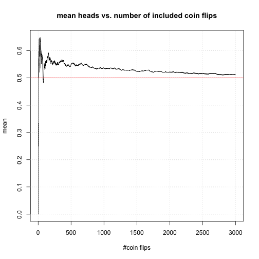
The figure shows that after 1000 coin tosses the mean is already fairly close to the actual probability and fluctuates only a little. The decrease in fluctuation is due to the fact that individual outcomes lose relative influence on the average as the number of trials increases:
When calculating the mean for a list of values \(x = {x_1, x_2, …, x_n}\), the denominator \(n\) corresponds to the number of trials (coin flips) whereas the numerator is the sum of all outcomes.
This can be rewritten as
In this sum each entry receives a weight of \(\frac{1}{n}\). Therefore the relative influence of each value shrinks with each new sample which explains the decreasing fluctuation.
But can such observations justify drawing conclusions about the actual bias/fairness of a coin?
Binomial Experiments
A single coin toss is an experiment with two possible outcomes. This kind of single binary trial is also known as a Bernoulli experiment. Repeated coin tossing, i.e. concatenating multiple Bernoulli experiments, is one instance of a so called binomial experiment.
Earlier we observed that the average of a binomial experiment approaches the actual bias of the variable of interest (e.g. the probability of a coin to land showing heads) as the number of trials increases. However, we still lack a notion of (un-)certainty about such estimates.
Let us have a look at what happens if we calculate the means of multiple independent binomial experiments.
BinomMeans <- function(experiments = 10000, coinTosses = 1000, p = 0.5) {
  # function to collect the mean outcomes of multiple binomial experiments
  #
  # Args:
  #  experiments: number of experiments
  #  coinTosses:  number of trials per experiment
  #  p:           proportion of 1s
  #
  # Returns:
  #  means: mean outcomes of multiple binomial experiments

  means <- c(NA)   # make a list to store the mean values
  length(means) <- experiments # allocate memory to store the mean values
  for (i in 1:experiments) { # for each experiment
    # flip a coin multiple times and store the average number of
    # 1's in a list
    means[i] <- mean(sample(x = c(1, 0), size = coinTosses,
                            replace = TRUE, prob = c(p,1-p)))
  }
  return(means)
}
We make a histograms of 100 means that are all based on 10000 independent fair coin tosses.
# 1000 means of 10000 coin tosses each
means100Exp <- BinomMeans(experiments = 100, coinTosses = 10000, p = 0.5)

# show histograms of the collected means
hist(means100Exp, breaks = 42, freq = FALSE)
abline(v = 0.5, col = "red") # draw vertical line at actual bias
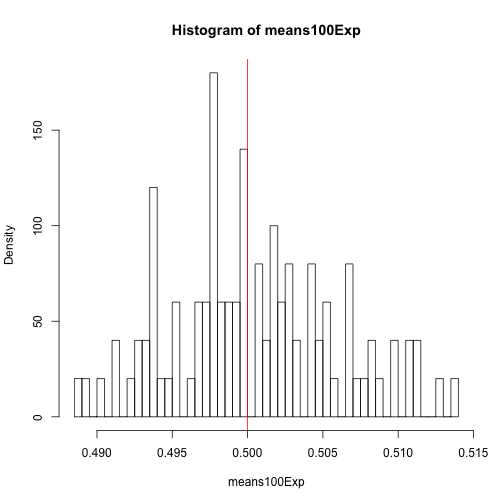
The means are scattered around the actual bias but it seems that there is a tendency towards the center.
To have more clarity we make the computer work a little harder:
10000 means of 1000 coin tosses each!
# 10000 means of 1000 coin tosses each. This may take a few seconds.
means10000Exp <- BinomMeans(experiments = 10000, coinTosses = 1000, p = 0.5)
# show histograms of the collected means
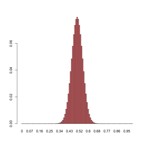
hist(means10000Exp, breaks = 42, freq = FALSE)
abline(v = 0.5, col = "red")
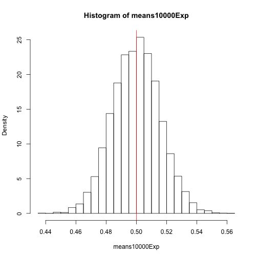
This distribution no longer looks arbitrary. In fact, it appears to resemble a discrete version of what some of you may remember as the normal or gaussian distribution.
But why does the distribution of mean values start taking this particular shape as the number of samples increases?
From Possibilities to Probabilities
The above approximate distribution does not only appear after a lot of coin flipping but is actually a property that directly arises from the number of ways in which particular events can occur.
If we flip a fair coin once there are two possible outcomes, heads h and tails t with equal probabilities of \(\frac{1}{2}\).
If we flip the coin twice we get one of the three following outcomes:
hh, tt, ht. However, not taking the order into account, there is only one way each for hh and tt to occur but there are two ways in which ht can occur (ht and th).
Accordingly, the probabilities of hh and tt are only \(\frac{1}{2} \cdot \frac{1}{2} = \frac{1}{4}\) each whereas the probability of ht is \(2 \cdot \left(\frac{1}{2} \cdot \frac{1}{2}\right) = \frac{1}{2}\).
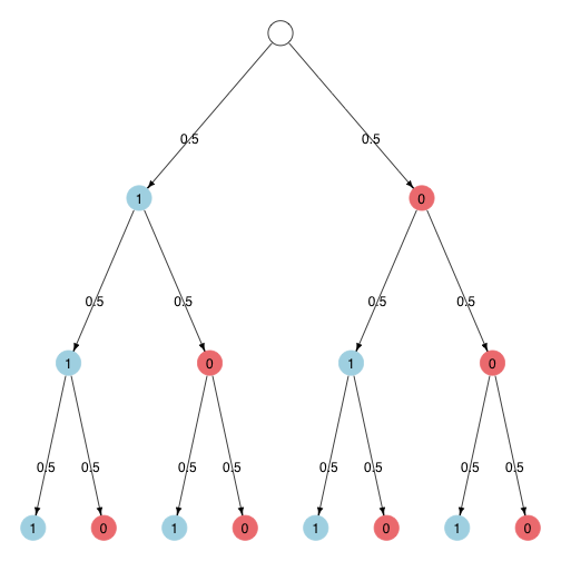
We can also illustrate this concept in a graph where the number of paths that lead to a node corresponds to the number of possible cases in which a particular distribution of heads and tails can occur.
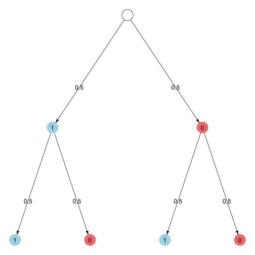
This graph represents the possible outcomes of a binomial experiment with two trials. You can think about it as showing the possible outcomes of two subsequent coin flips where “1” stands for one side and “0” for the other side of the coin.
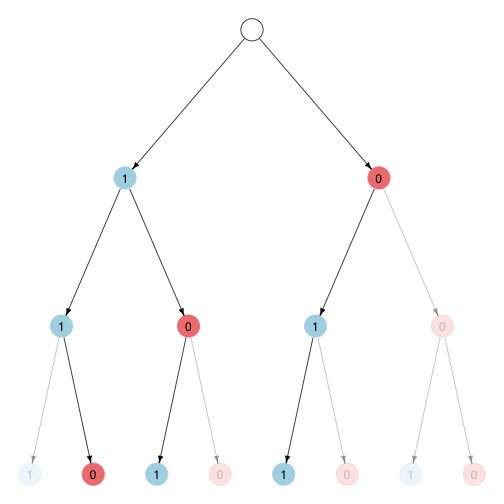
Similarly with three coin flips we have 4 possible outcomes out of which two (hhh and ttt) have the probability \(\frac{1}{2} \cdot \frac{1}{2} \cdot \frac{1}{2} = \frac{1}{8}\) and two (hht and tth) have the probability \(3 \cdot \left(\frac{1}{2} \cdot \frac{1}{2} \cdot \frac{1}{2}\right) = \frac{3}{8}\).
The Pascal Triangle
There is another graphical representation which makes determining the number of possible paths leading to a node even easier.
Take a look at the following graph:
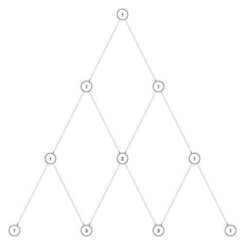
In this type of graph which is known as pascal triangle, each node is labeled with the number of paths that lead to it. The label of a node is also the sum of the values of the direct parent nodes when the value of the first parent is 1 because the number of paths that lead to a node corresponds to the sum of the number of paths leading to each of its parent nodes.
A transition towards a new node is always assigned to one of two possible outcomes (such as sides of a coin) depending on whether the new node is on the lower left or right of its parent node. Therefore, by simply following one path leading to a certain node and keeping track how many transitions go left and right one can infer the event which the node represents.
For instance, the first node labeled with a ‘3’ in the above example can only be reached by a combination of two left transitions and one right transition and thus represents the event (l, l, r), (h, h, t), or (1, 1, 0).
The Binomial Coefficient
The value of a node in the pascal triangle can also be calculated using the formula for the binomial coefficient.
The binomial coefficient is defined as
The notation \(\binom{n}{k}\) does not correspond to a traditional vector but can instead be understood as representing the number of ways to get exactly k successes (outcomes of one type) in n independent bernoulli trials.
Translated to the coin example this becomes the number of ways to get k heads in n independent coin tosses.
Example:
\(\binom{3}{2} = 3\): There are 3 possible ways in which three coin tosses could produce exactly two heads.
To calculate the binomial coefficient in R one can use the function choose(n, k).
choose(3, 2)
## [1] 3
So how does the size of a binomial experiment influence the distribution of possible paths which realise individual events?
Take a look at individual rows of the following Pascal Triangle:
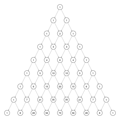
Nodes near the center of a row can be reached in many more ways than nodes on the edges. This means that there are more ways to have a balanced number of left and right transitions than uneven combinations.
Let’s have a look at the histograms for the values in some of these rows.
BinomHist <- function(n = 3, relative = FALSE) {
  # plot histogram of possible path counts for different success ratios
  # in an unbiased binomial experiment with sample size n
  #
  # Args:
  #  n:        integer, sample size
  #  relative: boolean, TRUE for relative path counts, FALSE for absolute

  # ways to get 0:n successes in n independent bernoulli experiments
  paths <- choose(n, 0:n) # use binomial coefficient for path counting
  if (relative == TRUE) {
    paths <- paths/(2^n) # normalize counts if requested
  }
  ratios <- c(0:n)/n # x-axis shows success ratios
  barplot(height = paths, names.arg = ratios,
          main = paste("Path distribution of L/R ratios,\n",
                       "n = ", n),
          xlab = "left/right ratio",
          ylab = ifelse(relative == TRUE,
                        "Relative number of paths", "Number of paths"),
          col = "lightblue")
}

# Show histograms for different sample sizes
#par(mfrow = c(2, 2))
BinomHist(5, FALSE)
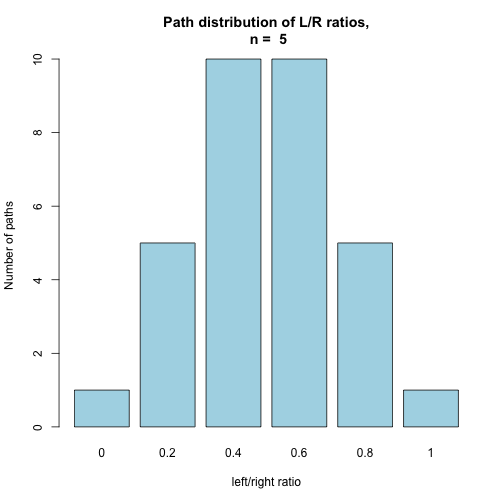
BinomHist(10, FALSE)
BinomHist(30, TRUE) # show relative number of paths for large n
BinomHist(100, TRUE)
Does this look familiar?
Each of these histograms represents the distribution of possible paths for different success ratios in a binomial experiment in which p = 0.5. When the counts are normalized to add up to one, their distribution can be interpreted as the probability distribution of the success ratio of n fair trials (coin flips).
In the previously observed distribution of fair coin outcome ratios, the use of this probability distribution can be seen in action. As the number of trials grows, the distribution appears naturally simply due to differences in the number of possible realizations.
Biased Binomial Distributions
In the case of a fair coin, using this path-based approach appears sensible. But what can we do in case of biased binomial experiments?
For a biased coin, the probabilities for each of the possible outcomes need to be considered in calculating the number of possible ways in which an event can happen.
Fortunately there is an extension to the binomial coefficient which allows calculation of probabilities of events with any bias. This extension is known as the binomial distribution and it is defined as
This formula consists of:
- the binomial coefficient \(\binom{n}{k}\): the number of ways of distributing exactly
ksuccesses in a sequence ofnindependent bernoulli trials - \(p^k\): the probability of
ksuccessful trials where each success has an individual probability ofp - \((1-p)^{n-k}\): the probability of having
n-kunsuccessful trials
Using this formula, the probabilities for different ratios can be obtained for any underlying bias p.
In R the probability of a success ratio for a binomial experiment of a certain size and a certain event probability can be obtained with dbinom(k, n, prob).
The following example returns the probability of having two heads in 3 coin tosses with a fair coin:
dbinom(x = 2, size = 3, prob = 0.5)
## [1] 0.375
We can also use dbinom() to obtain a probability distribution for different success ratios:
#par(mfrow = c(3,1))
barplot(dbinom(x = 0:100, size = 100, prob = 0.5),
        names.arg = c(0:100)/100,
        col = "lightcoral")
Note that with prob = 0.5 this distribution is identical to the normalized 100s row of the pascal triangle visualized in an earlier histogram.
When changing the bias of the coin, the distribution shifts its center accordingly:
#par(mfrow = c(2,1))
n <- 50
x <- 0:n
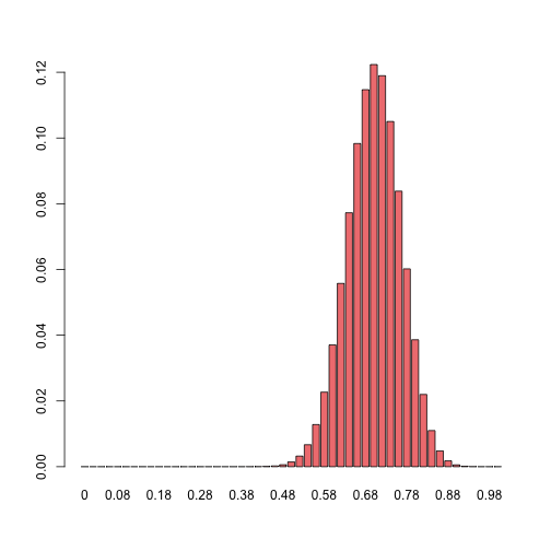
barplot(dbinom(x = x, size = n, prob = 0.7),
names.arg = x/n,
col = "lightcoral")
barplot(dbinom(x = x, size = n, prob = 0.3),
        names.arg = x/n,
        col = "lightcoral")
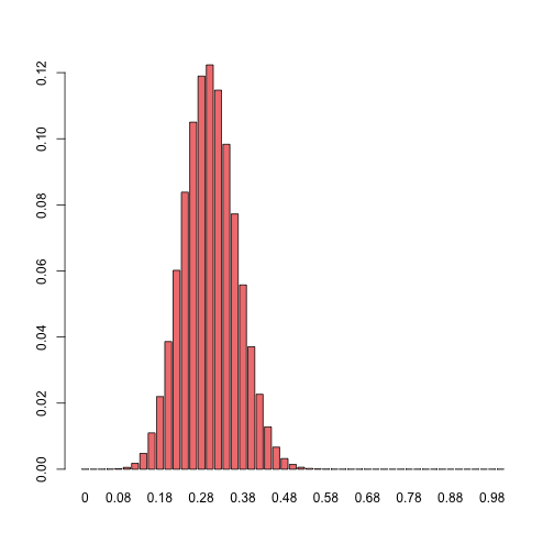
We can therefore assume that the sampling distribution of the mean for samples obtained with a biased coin will also have it’s center near the ratio that corresponds to the coin’s bias.
Biased Gold
Let us now take a look at the distribution of means we get from performing multiple sets of coin flips with our gold coin.
BinomMeansGold <- function(experiments, coinTosses) {
  # function to collect the mean outcomes of multiple binomial experiments
  # using an old gold coin
  #
  # Args:
  #  experiments: number of experiments
  #  coinTosses:  number of trials per experiment
  #
  # Returns:
  #  means: mean outcomes of multiple binomial experiments
  means <- c(NA)   # make a list to store the mean values
  length(means) <- experiments # allocate memory to store the mean values

  for (i in 1:experiments) { # for each experiment
    # flip a gold coin multiple times and store the average number of
    # 1's in a list
    means[i] <- mean(GoldCoinToss(coinTosses))
  }
  return(means)
}

# collect mean values of 10000 x 1000 coin flips with the old gold coin
# The Shape of the distribution dependents on number of experiments
# and the width is dependent on the number of coing tosses per experiment.
goldMeans <- BinomMeansGold(experiments = 10000, coinTosses = 1000)

# show histograms of the collected means
hist(goldMeans, breaks = 50, freq = FALSE, col = "gold")
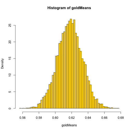
This distribution of mean outcomes suggests that this gold coin is more likely to land on one side than the other with a bias of around 0.618.
Because of our knowledge about the shape of binomial probability distributions we might be fairly confident that this bias is close to the true bias of the coin.
However, in real life it is sometimes not possible to repeat an experiment thousands of times in order to replicate the probability distribution of a random variable.
In a future post I will write about some approaches which are used for making inferences even with relatively small sample sizes.